ApartmentPredictor: Evaluation an Linear Regression

The script is now "code complete" - I think that the code works, but I haven't verified it yet.

The bitmap below reflects whether or not the model contains some features (whether some theta values always should be zero or not):

One test run of the model looks like this:

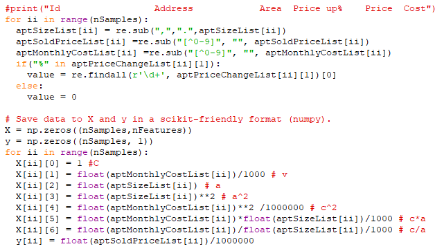
First, some characteristics of the y data set (final prices)
The bitmap reflects which of the features should be included in the model.
The MSE and MAE are shown for different sizes of training set/test set.
The best feature sets are recorded, both for MAE and MSE

The standard deviation of the price is 360 kSEK. When training different sets of features for different training sizes, the Medium Absolute Error is between 210 kSEK and 280 kSEK.

For example, when using a bitmap of 1010101 (considering constant, cost, area^2 and cost/area) and training it for 40 samples and testing on 10 samples, the average MAE is 217 kSEK. In this case, I repeated each bitmap/training set size for 100 times. This means, that I can make better predictions on the final prices using this program, compared with just guessing.

For one specific apartment that is for sale, the model predicts 2.1 MSEK +/- 0.2 MSEK. Time will tell what the actual price will be.

How to Evaluate the Performance of Linear Regression 

Initially, the linear regression algorithm operates on some training data. It estimates the error by adjusting the parameters using the gradient. It is repeating that, over and over and over again. 

When this is done, one should use the model to make predictions, and to compare those predictions to the actual data.  

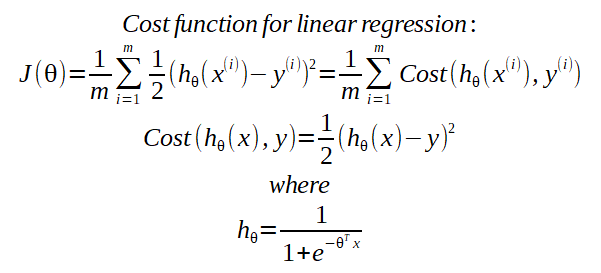
Error Metrics - There are several ways to estimate errors of predictions. There are plenty of articles that are discussing which to use and when. I'll compare both the Mean Squared Error and the Mean Absolute Error. 

The advantage of MSE is that it will punish big errors but on the other hand, it is not so robust to outliers.

Number of Features

The simulations suggest that there is no big difference between different sets of features, except some poor combinations. For example, using only the constant gave a pretty bad predictor with an MAE of 280 kSEK.

Size of Training Set
A machine learning application would need thousands, if not millions of data.

For apartments, there are two ways to increase the number of examples:

• Use a larger geographical area. The problem is that prices depend on the location, which would add complexity to the model. Two similar apartments will have very different prices, depending on their address.
• Use a longer time interval. This is also tricky - a data set covering a longer period of several years will be affected by price changes in the market.

I'm afraid that I'll have to live with the imperfection in the model.

This concludes the project ApartmentPredictor. For the next blog post, I'll focus on stocks again.

ApartmentPredictor: A Simple Logistic Regression Price Predictor (1)

Problem:
I want to predict apartment prices for a given area using the size and the monthly cost, using a regression model with statistics for sold apartments in a specified area.

It is fairly simple to get a sample of past apartment deals for an area using some real estate listings.

Preparing the Data
I created a web scraper in python that is using Regular Expressions and the Requests package.

In this data set, the Price reflects the final price agreed between the seller and the buyer.

The next step is to prepare the data for the SciKit package in Python. I will use two features (area and cost) to construct a model of seven parameters to optimize for:

I created two numpy arrays for the raw data:

• X (number of past apartment deals, number of features) 
• y (number of past apartment deals)

The Panda dataframe is populated by the two arrays:

The result is:

The data set's properties are:

Most of the features are derived from Cost and Area

So, just guessing that the final price would be the mean price would give an average error of 347 kSEK. This will be a measure of the model's performance: I hope that it will generate a lower error than 347 kSEK.

In the next blog post, I'll use SciKit to generate an initial prediction and evaluate that one.

Tools that I use:
SciKit  is a popular package for data analysis, data mining and machine learning. I use the linear regression.
Panda is popular for machine learning too. It makes it easy to organize data
Numpy is useful for matrices, linear algebra and organizing data.

Thanks Nagesh for the inspiring article.

Machine Learning: Lecture Notes (Week 9)

Gaussian Distribution (Normal Distribution) is used for anomaly detection. I'm quite familiar with this so I won't discuss this in my blog.

The Parameter Distribution Problem
Given a data set, estimate which distribution gave this data set using the Maximum Likelihood method:

• Estimate that the average (mu) to be the same as the average.
• Estimate that the variance (sigma) to be the same as the standard error squared.

Anomaly Detection Algorithm
Given a training set of m samples, each with n features, where the samples follow the normal distribution, p(x) can be calculated as:

• Choose features that might indicate anomalous examples.
• Fit parameters for the different features such as mean values and variance.
• Calculate p(x). If p(x) is smaller than a threshold, an anomaly is detected.

Put simply, the likelihood for one example is calculated. If that likelihood is too small, we probably have an anomaly.

This is the last lecture note for this course, since I've completed the course. The next blog post will discuss a simple logistic regression example for apartment prices.

Machine Learning: Lecture Notes (Week 8)

Unsupervised Learning
Unsupervised learning is training on a training set X without labels y.

Clustering algorithms finds clusters of similar features.

K-means
K-means is the most popular clustering algorithm.

It takes two random points as cluster centroids.

• Ignore the bias feature.
• Repeat:
• For each sample in the training set, it assigns it to the closest centroid.
• Each centroid is moved to the average location of its assigned training samples.

Optimization Objective
K-means can get stuck in a local optimum. Use random initialization several time to overcome this.

Elbow method for selecting number of clusters.

Create a curve of the cost function versus the number of clusters. The "elbow" will indicate the suitable number of clusters.

It can be necessary to reduce the number of features. Sometimes, features can be seen as redundant.

This can be done by projecting data from a set of higher dimensions to a plane of lower dimensions.

Principal Component Analysis

PCA tries to reduce the error between the data points and its projections.

PCA should not be confused with liner regression

Start with mean normalization (subtracting average from each value). The scale of features must be on a comparable scale.

Calculate coviarance matrix SIGMA = 1/m x^i {x^i}^T

Compute Eigenvectors U, S, V of SIGMA using singular value decomposition (SVD)

This gives U, a matrix of n column vectors. The first k column vectors are the new planes for the PCA.

U_reduce = U(1:k,:)

z=U_reduce^T x

Restoring:

X_approx = U_reduce x

Anomaly Detection - when to use

Use AD when there are few positive examples

Many different and unpredictable types of anomalies.

What features to use?

Use histograms to see whether it is a gaussian feature or not. If it is gaussian, it is suitable for anomaly detection. If it isn't, transform it to a gaussian distribution.

Recommender Systems

One approach can be to use a version of a regression analysis.

Collaborative Filtering

In this case, we don't have any information about the movies, such as romance/action etc. The users has specified which movies they like (theta values).

Alternate optimizing for indata and model parameters to get lower errors.

1. Initialize x and theta to smal random values.

2. Minimize J(x, theta) using gradient descent

Machine Learning: Lecture Notes (Week 7)

Support Vector Machine (SVM)
The cost function will be modified compared to the sigmod function. It will consist of a constant slope session and a constant session.

In SVM, the parameters CA+B shall be minimized. A is the cost term, B is the regularization term and C controls the weight between them.

When training the hypothesis function, the hypothesis (theta multiplied by input data) shall be

• Cost1: Bigger than 1, if y = 1
• Cost0: Smaller than -1, if y = 1

Support Vector Machine
Define f as a similarity function that calculates the proximity to landmarks (combinations of feature values):

The function is based on a Gaussian kernel. Sigma affects the pointyness of the curve - a small sigma means a pointier curve.

Big C (small lambda): Low bias, high variance. Optimizing training set.
Small C (big lambda): High bias, low variance. Optimizing to reduce overfitting.

Machine Learning: Lecture Notes (Week 6)

Machine Learning Diagnostics
When getting poor test results from a trained machine learning algorithm, some solutions are available:

• More training examples
• More/less features
• Higher/smaller training rate
• Adding polynomial features

The challenge is how to find which of the solutions will help out in a particular project.

Machine Learning Diagnostics are tests that can help narrowing down which actions listed above may help improving the performance of a ML project.

How to Evaluate a Hypothesis
A hypothesis should be able to generalize to new examples that aren't in the training set. An over fitted system will preform poorly with respect to this.

One way of verifying a hypothesis is to divide the dataset into a training set and a test set. After training a neural network, apply the hypothesis to the test set and check whether the error is acceptable. ~70% of data can be training set.

Model Selection with Train/Validation/Test sets
Degree of polynomial for regression can be determined by fitting the training data to a set of polynomials with different degrees. By evaluating the polynomials on a test set, a model is selected. However, that may not be a good generalization since that polynomial is fitted to the test set (the parameter d) and may not be generalized enough.

Instead, divide the data set into three parts:

• Training set ~60%
• Cross validation set (CV) ~20%
• Test set ~20%

Calculate corresponding cost functions.

Train the data to minimize the training set cost function. Test the models using the cross validation set and select the model with the lowest  cross validation error. Estimate the error using the test set.

Bias vs Variance
High Bias - Underfit
High Variance - Overfit

Calculate the Training and Cross Validation error. Plot error vs degree of polynomial.

Bias: Both training and CV errors are high
Variance: CV errors are high, but training errors are low.

Regularization
For a polynomial as a hypothesis, a high value for lambda (regularization) implies that all non-bias parameters will be close to zero. A low value for lambda gives an overfitted system. How to chose the regularization parameter?

• Calculate the cost functions for the training set, the cross validation set and the test set (mean-square error).
• Try different lambdas (doubling each step) and minimize the cost functions. 
• Use the cross validation set and check which of them has the lowest error on the cross validation set.
• Finally, calculate the test error on the test data.

Readers that follow the course may note that I've omitted some parts of the lectures. I am doing that for a pragmatic reason - time. I take these notes in order to help me remember (rubberduck) the important lessons. If you want better coverage of the course. I recommend taking the course.

Machine Learning: Lecture Notes (Week 5)

In Neural Networks, backpropagation is the process of minimizing the cost function by adjusting the elements in the different layers.

This is done in a similar way as in linear regression. I calculate the partial derivatives of the cost function:

The Back Propagation Algorithm:
Given a training set:

z is the output, a is the activation value.

Set deltas to zero for all layers, and their respective input and output nodes.

Repeat for all training examples:
Forward propagation:
Set the initial activation values to a(1) = x(i).
Calculate the activation values for all layers using forward propagation.

CONTINUE!!!
Now, calculate the errors by a(L)-y(i)
Delta is set to delta + the activation value miltiplied by the error.

Machine Learning: Lecture Notes (week 4/5)/Neural Networks

My earlier blog posts on Neural Networks are here.

Neural Networks are suitable for more non-linear representations. When the feature set gets bigger, the polynomial will be unreasonably big.

Terminology:

The course considers two types of classification: Binary and Multi-class classification.

The cost function will be a generalisation of the cost function for logistic regression. For the multi-class case, the cost function will be calculated for each output.

Back Propagation - Cost Function

Back propagation starts with calculating the error of the last hidden layer (L-1). Using that, the second last hidden layer (L-2) can be estimated etc, back to the first layer.

The cost function for neural networks is more complex than the cost function for regularized logistic regressions, with a couple of nested summations.

Let's look at the summations:

• The first summation spans over the training set. This is similar to the logistic regression.
• The second summation spans over the output nodes. This means that the cost function must consider all different output bins.
• The first summation in the regularization term spans over all layers:
• The second summation in the regularization term spans over all the input nodes in the current layer, including bias unit (number of columns in the matrix)
• The third summation in the regularization terms spans over all the output nodes in the current layer, excluding the bias unit (number of rows in the matrix)

Machine Learning: Lecture Notes (week 3)

These are some lecture notes from the third week of the online Machine Learning Course at Stanford University.

Classification
Many machine learning problems are concerning Classification. That may be "dirty/clean", malignant/benign tumor, spam/no spam email etc.

In this case, the training output y will be either zero (negative class) or one (positive class) for the two class case.

Logistic Regression / Hypothesis Representation
Logistic regression model is improved with a sigmoid function:

The sigmoid function offers a smooth transition from 0 (z << 0) to 1 (z >> 0).

h_θ(x) is the probability for a positive result, given the input x.

Decision Boundary
A decision boundary is the limit between the set of x that results in h_θ(x)>0.5 and the set of h_θ(x)<0.5

Cost Function

This cost function will give zero cost, if the hypothesis is correct and an infinite cost, if the hypothesis is incorrect.


Simplified Cost Function and Gradient Descent
For the two binary cases for the cost function (y=0 and y=1), the cost function can be written as:

This function be derived using maximum likelihood estimation.

The optimization problem is now to minimize J with respect to the parameters and the observations.

The gradient descent method will update the parameters with the error multiplied by the observations:

Advanced Optimization
Another optimization algorithms are

1. Gradient Descent
2. Conjugate Gradient
3. BFGS
4. L-BFGS

2-4 doesn't need to select alpha (learning rate) and are often faster than gradient descent. They are also more complex.

Regularization
Too many features in the hypothesis may cause overfitting. That means that the model fits the training set perfectly but misses out in new cases. There are two ways to handle overfitting:

• Reducing number of features (manually or using a selection algorithm)
• Regularization (keep all features but reduce magnitude of theta)

Regularization will add the sizes of some hypothesis parameters to the cost function. The first theta parameter will not be optimized by convention.

The vector form will be:

Machine Learning: Lecture Notes (1)

Here are some lecture notes from the second week of the online Stanford course in Machine Learning. I take the notes for myself as a form of rubberducking.

Terminology from week 1 (single feature linear regression):

• m is the number of training examples. 
• n is the number of features.   
• y is the output from the training set 
• x are the input features in the training set
• x⁽ⁱ⁾ are the input features of the i^th training set. 
• h_θ =>θ₀+θ₁x₁ + ... + θ_nx_n is the hypothesis function that will be modified to fit the training set.
• θ_j are the hypothesis values for each feature.
• J is the cost function. A common cost function is the mean square error function
• α is the learning rate

Multiple features:

It is common to add a constant feature to the model: θ₀, where x₀ = 1
Using matrices, h_θ (x) = θ^Tx
Gradient Descent Algorithm
For each θ_j: 
    Add the derivative of the cost function for that feature
    Add α times the average of the (hypothesis minus the actual observation) multiplied by that feature value.
Gradient Descent - Feature Scaling
The gradient descent algorithm can converge quicker if the feature range are scaled to the same interval.
Feature scaling is dividing the input variables by the range of the input variables. The new range will be 1, but the values can still be higher.

Mean normalization means subtracting the mean from each value. If you combine those methods, you get:

x_i := (x_i - mean(x))/range(x)

Normal Equation
This is a way to minimize J without iterations.

Gradient Descent or Normal Equation
GD: Need to chose a learning rate. NE: No need to choose a learning rate.
GD: Needs many iterations. NE: Needs no iterations
GD: O(kn^2). NE: O(n^3). NE is heavy for large feature sets!


The next step is a programming assignment where I'll implement linear regression to a simple data set. I won't publish that on my blog, however.

Machine Learning: Online Stanford Course

I have spent some time on programming this week - but not on my pet projects.

For obvious reasons, I can't elaborate on the programming I've done at work more that I have learnt a lot.

I've joined a dojo excercise on Machine Learning with an online course from Stanford/Coursera. We followed an example where we implemented a simple linear regression.

So far, I think the course is good for a beginner in AI. I seriously consider purchasing a course certificate when I finish that course.

StockReader: White and Black Lists

As I mentioned in earlier blog posts, I want to have a black list and a white list for combinations of expected name and returned names. Now, I got that code working.

An XML file lists all valid combinations (white list) and invalid combinations (black list). When the program is started, that XML file is opened and the lists are read into two dictionaries.

When the program finds a new stock record, it will query the class nameChecker for the combination of the expected name and the returned name. The result will be one of the following:

• Found in white list: The record can be added to the database
• Found in black list: The record is faulty and will be discarded.
• Found in neither white or black list: The combination needs to be assessed by the user manually. The record won't be added to the database. Instead, a proposal xml string is printed to the console when the scanning of records is done.

One of the few methods that is properly commented.
I really need to refactor my code.

The output can be copied into the XML file for the next iteration:

This means that there will be a lot of manual work initially. Once the lists are updated, unknown mismatches will be less frequent.

The current version of the web scraper builds the list of stocks dynamically and mismatches should be very unlikely.

Side Note: I'm focusing more on programming tasks at work. Therefore, I'll have a slower pace on my spare time projects and sometimes, I'll update the blog every second week, instead of every week.

StockAnalyzer: Adding XML Reader to the Program

I've created a separate page for StockReader and StockAnalyzer, with a short summary of the programs. In this blog post, I'll use XML and C# dictionaries to verify that the stock names are correct for the stock records.

When feeding the stock records from the csv files, I need to verify whether the stock name I queried (the first string) matches the actual stock record that I got (the second string).

As I mentioned in my last post, I'll have three lists of valid, invalid and unknown combinations in a XML file. The program will read that file and populate corresponding dictionaries.

When the program reads a stock record, it will look for the stock names in the dictionaries.

• If it is found in the white list, that stock record can be added to the database.
• If it is found in the black list, that stock record is ignored.
• Otherwise, the program will print a recommended xml tag. The user can decide on whether to add that tag to the white or black list.

The user will edit the XML file and move combinations from the gray list to the black or white list manually.

XMLReader vs XMLDocument in C#
XMLReader is a read-only representation of the XMLDocument. The reader requires more code but is less memory consuming. I've decided to use the XML

New Class: NameChecker
The name checking will be handled in a separate class, that is called from fileParser. I'll implement it in the next post.

Mapping the Wanted Stock Name to the fetched Stock Name
In C#, there is no mapping from value to key in dictionaries. Key to value mappings are smooth. Therefore, searching for the key will be time consuming.

I'll use the dictionaries to search for the key (the fetched values). This will give a list of values that represent the wanted values (most of the cases one value).

StockAnalyzer: Handling Stock Name Mismathes

One early flaw of the earlier versions of my webscraper was that it used hard coded links when retrieving the stock data. The links were based on hard coded numbers and I needed a safeguard check to detect if those numbers changed.

The program took the first Name ("Eniro") as the stock name. It used the corresponding numbers (869, 2398 and 46100341) to build three URL strings to fetch the stock data.

For that reason, I had the stock name as the two first entries: The first name is the stock that I want to fetch and the second name is the stock that was actually collected. Ideally, the names matched each other, but there are several mismatches.

I need to verify the stock records before adding them to the database. One check will be to see whether the first string is "---Void---" or not. That string was a placeholder and that record shall be discarded.

Further, I need to check whether the stock data I have really matches the stock name or not. To do this, I'll use a XML file that contains three lists:

• White List for the allowed combinations of names,
• Grey List for the combinations of names that hasn't been verified by the user yet and
• Black List for the illegal combinations of names (these records will be ignored by the program).

A lesson learnt from this is to make sure that the web scraped data is in a good shape already when scraping. The next blog post will cover some XML topics for CSharp.

Garage Cleanup

My summer project at the summer cottage was to fix the garage. You can see the before images below.

 The black marks in the wall are probably from car decks. There is also a couple of holes in the wall.

 After throwing away some rubbish and emptying the garage, I was able to paint the surfaces. I got help with painting the kitchen shelves (they are from a French kitchen of the late 1970's).

I've mounted four connected IKEA Hejne shelves on the far wall. To avoid stains from the firewood, I had a tarp behind the wood.

 And two connected 50 cm IKEA Hejne shelves in the corner.

This took some time from my ordinary pet projects. I'll resume them now.

StockAnalyzer: Lessons Learned from Web Scraping

After spending too many hours fixing flawed data, I've learnt some lessons:

Use English when describing the data
Using another language is a very common mistake for non-English natives, especially if one believes that the data will have a very limited audience. Applications has a tendency to grow and involve more people.

Use standardized formats for input data
I've seen some strange data files for other applications, and it is a nightmare to decode them. Unless there are strong reasons to save storage space, I recommend using plain text files such as:

• csv - Compact for data. However, missing separators will shift all data to the left. This can be difficult to recover
• json - Quite compact for data, but slightly harder to implement. This way, it is clear what the different values represent.
• xml - This will generate some overhead and may be difficult to implement, unless there is some handy xml class that can handle the xml coding.
• Database - Feeding the scraped data directly into a database. This is a bit complex but has some advantages: It will indicate if there are errors, the data labeling is clear and it will be compact. One disadvantage is that it takes some time to set up the database.

Handle bad or missing data directly
If there are flaws in the web scraper, or the web server, the data will be flawed. This will be a big problem if the web scraping continues - big chunks of data may be missing or erroneous.

Test the data and the format
This will help finding flawed data early. Tests may check the number of data points, the type of data (integer/float/names) and how the data is changing over time.

Cross-verify numbers
It can be useful to scrape some extra data for cross-checks. For example, scraping Price, Earnings and Price/Earnings will make it easy to check that those values are valid.

Handle changes in the data
This is quite obvious. The web services that you want to scrape will change its interface once in a while and that will break your web scraper. As mentioned above, you need to see that immediately, otherwise you'll have tonnes of data that needs to be fixed.

Automate the web scraping
After all, the purpose of computers is to liberate people from manual labor. This applies to web scraping too. If it isn't started automatically, it is easy to forget it.

It is easy to set up the web scraping script using cron (Linux) or the Task Scheduler. I strongly recommend that you check that the tasks are really started as they should, at least the Task Scheduler isn't totally reliable.

Make the data database-friendly
It is very likely that you will send the data to a database sooner or later. Considering how to do that early will save you a lot of effort.

Side note:
One very common issue is missing yield values. That can span over several months of data. I've created a python script to resolve that issue by adding an empty piece of data for the missing piece of information.

StockAnalyzer: Fixing Flawed Data (continued)

My work on the program StockAnalyser is currently in a iterative cycle:

• The program adds records to the database until it crashes because of some flaw in the input data
• Fix that issue 
• Repeat

This means that most of the blog posts for now focus on handling new cases of flawed input data. Please bare with me.

Each record is a line of comma separated values. For some records, one value is missing. By looking at the remaining data, I'm able to see what data is missing and replace that manually.

By adding a semicolon before the profit margin (in this case), the program will be able to populate the missing data with a null value.

Fixing hundreds, or thousands of records isn't possible to do by hand, and I'll need to create a script that can re-populate the missing data. I'll develop that script in the next blog post.

StockAnalyser: Recovering Missing Data

In this blog post, I'll add code that protects the program when parsing strings to float values and I'll also add code that tries to recover missing information.

First, I'll add try-catch clauses to handle parsing errors from string to floats.

After that, I'll add functions to verify and populate null entries of the key numbers.

For the triplet of P, P/E and E. there are eight possible scenarios:

P = null, P/E = null and E = null - Impossible to recover

P = null, P/E = null and E != null -Impossible to recover

P = null, P/E != null and E = null - Impossible to recover

P = null, P/E != null and E != null - Recover P

P != null, P/E = null and E = null - Impossible to recover

P != null, P/E = null and E = !null - Recover P/E

P != null, P/E != null and E = null - Recover E

P != null, P/E != null and E != null - No need to recover

I'll start to count how many null values I have. If there are two or more null values, I can't recover any data. If there is no null value at all, I don't need to recover any data.

I will add two boolean flags later.
One will indicate if any data in the stock record has been recovered and
 another flag will indicate if the data is so bad that it shouldn't be sent into the database.

The screen shot below illustrates how the earning value is recovered (example from 2018-06-13, AAK, a Swedish company that is producing vegetable oil and fat.)

Similar functions are added for the Price, Price per Capital (P/JEK) and the Capital per share.

Now, only profit margin is missing. Since that is calculated as the profit (P) divided by the total revenue (not recorded), I can't recover that value. I'll simply parse "Null" to the database, if that is missing.

After fixing this, I was able to scan stocks until 2019-02-15. For that date, most of the information is missing.

The fix here is to add a flag that indicates whether the stock record contains sufficient information to be added to the database. 

Side note: The board of AAK decided to perform a 6:1 share split, where one old share generated six new shares. This explains why some data was missing for that date. The next project will detect and handle share splits.