ApartmentPredictor: A Simple Logistic Regression Price Predictor (1)

Problem:
I want to predict apartment prices for a given area using the size and the monthly cost, using a regression model with statistics for sold apartments in a specified area.

It is fairly simple to get a sample of past apartment deals for an area using some real estate listings.

Preparing the Data
I created a web scraper in python that is using Regular Expressions and the Requests package.

In this data set, the Price reflects the final price agreed between the seller and the buyer.

The next step is to prepare the data for the SciKit package in Python. I will use two features (area and cost) to construct a model of seven parameters to optimize for:

I created two numpy arrays for the raw data:

• X (number of past apartment deals, number of features) 
• y (number of past apartment deals)

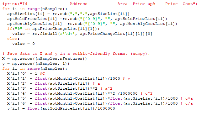
The Panda dataframe is populated by the two arrays:

The result is:

The data set's properties are:

Most of the features are derived from Cost and Area

So, just guessing that the final price would be the mean price would give an average error of 347 kSEK. This will be a measure of the model's performance: I hope that it will generate a lower error than 347 kSEK.

In the next blog post, I'll use SciKit to generate an initial prediction and evaluate that one.

Tools that I use:
SciKit  is a popular package for data analysis, data mining and machine learning. I use the linear regression.
Panda is popular for machine learning too. It makes it easy to organize data
Numpy is useful for matrices, linear algebra and organizing data.

Thanks Nagesh for the inspiring article.

Machine Learning: Lecture Notes (Week 9)

Gaussian Distribution (Normal Distribution) is used for anomaly detection. I'm quite familiar with this so I won't discuss this in my blog.

The Parameter Distribution Problem
Given a data set, estimate which distribution gave this data set using the Maximum Likelihood method:

• Estimate that the average (mu) to be the same as the average.
• Estimate that the variance (sigma) to be the same as the standard error squared.

Anomaly Detection Algorithm
Given a training set of m samples, each with n features, where the samples follow the normal distribution, p(x) can be calculated as:

• Choose features that might indicate anomalous examples.
• Fit parameters for the different features such as mean values and variance.
• Calculate p(x). If p(x) is smaller than a threshold, an anomaly is detected.

Put simply, the likelihood for one example is calculated. If that likelihood is too small, we probably have an anomaly.

This is the last lecture note for this course, since I've completed the course. The next blog post will discuss a simple logistic regression example for apartment prices.

Machine Learning: Lecture Notes (Week 8)

Unsupervised Learning
Unsupervised learning is training on a training set X without labels y.

Clustering algorithms finds clusters of similar features.

K-means
K-means is the most popular clustering algorithm.

It takes two random points as cluster centroids.

• Ignore the bias feature.
• Repeat:
• For each sample in the training set, it assigns it to the closest centroid.
• Each centroid is moved to the average location of its assigned training samples.

Optimization Objective
K-means can get stuck in a local optimum. Use random initialization several time to overcome this.

Elbow method for selecting number of clusters.

Create a curve of the cost function versus the number of clusters. The "elbow" will indicate the suitable number of clusters.

It can be necessary to reduce the number of features. Sometimes, features can be seen as redundant.

This can be done by projecting data from a set of higher dimensions to a plane of lower dimensions.

Principal Component Analysis

PCA tries to reduce the error between the data points and its projections.

PCA should not be confused with liner regression

Start with mean normalization (subtracting average from each value). The scale of features must be on a comparable scale.

Calculate coviarance matrix SIGMA = 1/m x^i {x^i}^T

Compute Eigenvectors U, S, V of SIGMA using singular value decomposition (SVD)

This gives U, a matrix of n column vectors. The first k column vectors are the new planes for the PCA.

U_reduce = U(1:k,:)

z=U_reduce^T x

Restoring:

X_approx = U_reduce x

Anomaly Detection - when to use

Use AD when there are few positive examples

Many different and unpredictable types of anomalies.

What features to use?

Use histograms to see whether it is a gaussian feature or not. If it is gaussian, it is suitable for anomaly detection. If it isn't, transform it to a gaussian distribution.

Recommender Systems

One approach can be to use a version of a regression analysis.

Collaborative Filtering

In this case, we don't have any information about the movies, such as romance/action etc. The users has specified which movies they like (theta values).

Alternate optimizing for indata and model parameters to get lower errors.

1. Initialize x and theta to smal random values.

2. Minimize J(x, theta) using gradient descent

Machine Learning: Lecture Notes (Week 7)

Support Vector Machine (SVM)
The cost function will be modified compared to the sigmod function. It will consist of a constant slope session and a constant session.

In SVM, the parameters CA+B shall be minimized. A is the cost term, B is the regularization term and C controls the weight between them.

When training the hypothesis function, the hypothesis (theta multiplied by input data) shall be

• Cost1: Bigger than 1, if y = 1
• Cost0: Smaller than -1, if y = 1

Support Vector Machine
Define f as a similarity function that calculates the proximity to landmarks (combinations of feature values):

The function is based on a Gaussian kernel. Sigma affects the pointyness of the curve - a small sigma means a pointier curve.

Big C (small lambda): Low bias, high variance. Optimizing training set.
Small C (big lambda): High bias, low variance. Optimizing to reduce overfitting.

Machine Learning: Lecture Notes (Week 6)

Machine Learning Diagnostics
When getting poor test results from a trained machine learning algorithm, some solutions are available:

• More training examples
• More/less features
• Higher/smaller training rate
• Adding polynomial features

The challenge is how to find which of the solutions will help out in a particular project.

Machine Learning Diagnostics are tests that can help narrowing down which actions listed above may help improving the performance of a ML project.

How to Evaluate a Hypothesis
A hypothesis should be able to generalize to new examples that aren't in the training set. An over fitted system will preform poorly with respect to this.

One way of verifying a hypothesis is to divide the dataset into a training set and a test set. After training a neural network, apply the hypothesis to the test set and check whether the error is acceptable. ~70% of data can be training set.

Model Selection with Train/Validation/Test sets
Degree of polynomial for regression can be determined by fitting the training data to a set of polynomials with different degrees. By evaluating the polynomials on a test set, a model is selected. However, that may not be a good generalization since that polynomial is fitted to the test set (the parameter d) and may not be generalized enough.

Instead, divide the data set into three parts:

• Training set ~60%
• Cross validation set (CV) ~20%
• Test set ~20%

Calculate corresponding cost functions.

Train the data to minimize the training set cost function. Test the models using the cross validation set and select the model with the lowest  cross validation error. Estimate the error using the test set.

Bias vs Variance
High Bias - Underfit
High Variance - Overfit

Calculate the Training and Cross Validation error. Plot error vs degree of polynomial.

Bias: Both training and CV errors are high
Variance: CV errors are high, but training errors are low.

Regularization
For a polynomial as a hypothesis, a high value for lambda (regularization) implies that all non-bias parameters will be close to zero. A low value for lambda gives an overfitted system. How to chose the regularization parameter?

• Calculate the cost functions for the training set, the cross validation set and the test set (mean-square error).
• Try different lambdas (doubling each step) and minimize the cost functions. 
• Use the cross validation set and check which of them has the lowest error on the cross validation set.
• Finally, calculate the test error on the test data.

Readers that follow the course may note that I've omitted some parts of the lectures. I am doing that for a pragmatic reason - time. I take these notes in order to help me remember (rubberduck) the important lessons. If you want better coverage of the course. I recommend taking the course.

Machine Learning: Lecture Notes (Week 5)

In Neural Networks, backpropagation is the process of minimizing the cost function by adjusting the elements in the different layers.

This is done in a similar way as in linear regression. I calculate the partial derivatives of the cost function:

The Back Propagation Algorithm:
Given a training set:

z is the output, a is the activation value.

Set deltas to zero for all layers, and their respective input and output nodes.

Repeat for all training examples:
Forward propagation:
Set the initial activation values to a(1) = x(i).
Calculate the activation values for all layers using forward propagation.

CONTINUE!!!
Now, calculate the errors by a(L)-y(i)
Delta is set to delta + the activation value miltiplied by the error.