Machine Learning: Lecture Notes (week 4/5)/Neural Networks

My earlier blog posts on Neural Networks are here.

Neural Networks are suitable for more non-linear representations. When the feature set gets bigger, the polynomial will be unreasonably big.

Terminology:

The course considers two types of classification: Binary and Multi-class classification.

The cost function will be a generalisation of the cost function for logistic regression. For the multi-class case, the cost function will be calculated for each output.

Back Propagation - Cost Function

Back propagation starts with calculating the error of the last hidden layer (L-1). Using that, the second last hidden layer (L-2) can be estimated etc, back to the first layer.

The cost function for neural networks is more complex than the cost function for regularized logistic regressions, with a couple of nested summations.

Let's look at the summations:

• The first summation spans over the training set. This is similar to the logistic regression.
• The second summation spans over the output nodes. This means that the cost function must consider all different output bins.
• The first summation in the regularization term spans over all layers:
• The second summation in the regularization term spans over all the input nodes in the current layer, including bias unit (number of columns in the matrix)
• The third summation in the regularization terms spans over all the output nodes in the current layer, excluding the bias unit (number of rows in the matrix)

Machine Learning: Lecture Notes (week 3)

These are some lecture notes from the third week of the online Machine Learning Course at Stanford University.

Classification
Many machine learning problems are concerning Classification. That may be "dirty/clean", malignant/benign tumor, spam/no spam email etc.

In this case, the training output y will be either zero (negative class) or one (positive class) for the two class case.

Logistic Regression / Hypothesis Representation
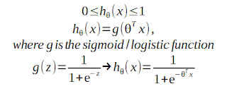
Logistic regression model is improved with a sigmoid function:

The sigmoid function offers a smooth transition from 0 (z << 0) to 1 (z >> 0).

h_θ(x) is the probability for a positive result, given the input x.

Decision Boundary
A decision boundary is the limit between the set of x that results in h_θ(x)>0.5 and the set of h_θ(x)<0.5

Cost Function

This cost function will give zero cost, if the hypothesis is correct and an infinite cost, if the hypothesis is incorrect.


Simplified Cost Function and Gradient Descent
For the two binary cases for the cost function (y=0 and y=1), the cost function can be written as:

This function be derived using maximum likelihood estimation.

The optimization problem is now to minimize J with respect to the parameters and the observations.

The gradient descent method will update the parameters with the error multiplied by the observations:

Advanced Optimization
Another optimization algorithms are

1. Gradient Descent
2. Conjugate Gradient
3. BFGS
4. L-BFGS

2-4 doesn't need to select alpha (learning rate) and are often faster than gradient descent. They are also more complex.

Regularization
Too many features in the hypothesis may cause overfitting. That means that the model fits the training set perfectly but misses out in new cases. There are two ways to handle overfitting:

• Reducing number of features (manually or using a selection algorithm)
• Regularization (keep all features but reduce magnitude of theta)

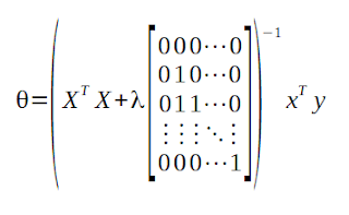
Regularization will add the sizes of some hypothesis parameters to the cost function. The first theta parameter will not be optimized by convention.

The vector form will be: